Introduction
For companies and investment funds holding a stock portfolio of more than 100 million dollars in value, the US stock exchange commission (SEC) requires a Form 13F filing. This document is filed each quarter and lists the stock holdings of the company for the last quarter. It is usually filed up to 45 days after the deadline of the reporting period with the SEC and is freely available from their databases.
E.g. https://www.sec.gov/cgi-bin/browse-edgar?action=getcompany&CIK=0001061768&owner=include&count=40
There are a few webpages who list the information of these filings (e.g. https://fintel.io or https://formthirteen.com/) but I thought it would be fun to create an own analysis tool that downloads and parses these filings and generates easy to read plots that show the quarterly changes in stock holdings.
Please evaluate the risks responsibly when investing in stocks as it should not be a form of gambling. Especially in 2020, where the markets have become unpredictably volatile.
Example Usage
This tool downloads SEC Form 13F filings for a company/fund from the SEC Edgar database in order to analyze changes in the stock portfolio.
To initialize:
- Import the class definition files.
- Look up the company identifier (CIK number).
- Specify the company name.
- Create a Portfolio object.
from Portfolio13FHR import Portfolio

CIK = '0001061768'
Name = 'Baupost Group LLC/MA'

portfolio = Portfolio(CIK,Name)
Upon creation, all latest SEC Form 13F filings are downloaded automatically into a folder in XML format and the BeautifulSoup package is used to parse the relevant information from the documents into DataFrames.
In order to compare the portfolio difference of the two most recent filings use the following methods:
portfolio.compare_recent_changes()
portfolio.data_recent.head()

portfolio.plot_recent_shares_change(portfolio.data_recent)
portfolio.plot_recent_value_change(portfolio.data_recent)

# Most recent additions
print("Recent portfolio additions: \n",portfolio.data_recent_additions[['value_current_perc','shares_change_perc']])
Recent portfolio additions:
                                value_current_perc  shares_change_perc
LIBERTY GLOBAL PLC (SHS CL C)                14.6                 1.6
QORVO INC                                     4.2                 0.1
TRANSLATE BIO INC                             4.0                 2.8
HD SUPPLY HLDGS INC                           2.9                 6.5
ATARA BIOTHERAPEUTICS INC                     1.8                19.4
HCA HEALTHCARE INC                            1.2               100.0
VENTAS INC                                    0.3               100.0
VERINT SYS INC                                0.3               100.0
SS&C TECHNOLOGIES HLDGS INC                   0.1               100.0
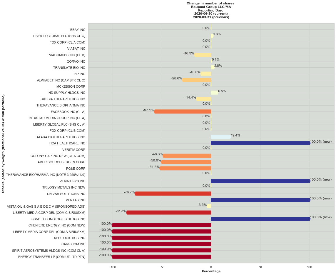
The first plot shows an overview based on the changes in Number of shares for the portfolio:
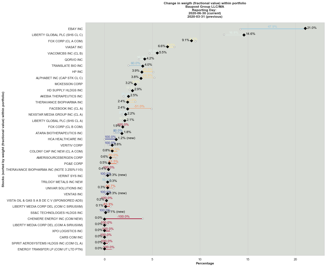
The second plot shows the changes in weights of the total portfolio value in the most recent filing (Note that this plot includes both the share purchases or sellings as well as the changes of the share price):
If desired, analyze a specific stock further using the “analyze_stock()” method:
# Dictionary of name to stock symbol
symbols = {
  'HCA HEALTHCARE INC': 'HCA'
}

OFFSET = 120 # Plot additional OFFSET days before start of reporting period
portfolio.analyze_stock('HCA HEALTHCARE INC', symbols['HCA HEALTHCARE INC'], PLOT_OFFSET=OFFSET)
The method downloads share price information using the YahooFinance API and creates a bokeh plot as html file with information on the minimum/maximum purchase price during the reporting period as well as the difference compared to the latest trading day:
Source Code
The complete code is available here: https://github.com/zpetan/sec-13f-portfolio-python
Code: Downloading and parsing from SEC Edgar Database
"""
Author: Pepe Tan
Date: 2020-10-06
MIT License
"""


import pandas as pd
from bs4 import BeautifulSoup
from ticker_class import Ticker
from datetime import datetime


class Filing13F:
    """
        Class containing common stock portfolio information from an institutional investor.
        1. Parsed from 13F-HR filing from SEC Edgar database.

    """

    # If True prints out results in console
    debug = False


    def __init__(self,filepath=''):
        """ Initialize object """
        self.filepath = filepath # Path of file

        # Directly call parse_file() when filepath is provided with __init__
        if self.filepath:
            self.parse_file(self.filepath)


    def parse_file(self, filepath=''):
        """ Parses relevant information from 13F-HR text file """
        self.filepath = filepath # Path of file

        if self.debug:
            print(self.filepath)

        # Opens document and passes to BeautifulSoup object.
        doc = open(filepath)
        soup = BeautifulSoup(doc, 'html.parser') # OBS! XML parser will not work with SEC txt format

        # Print document structure and tags in console
        if self.debug:
            print(soup.prettify())

            for tag in soup.find_all(True):
                print(tag.name)

        ## --- Parse content using tag strings from txt document: <tag> content </tag>
        # OBS html.parser uses tags in lowercase

        # Name of filing company
        self.company = soup.find('filingmanager').find('name').string
        # Company identifier: Central Index Key
        self.CIK = soup.find('cik').string
        # Form type: 13F-HR
        self.formtype = soup.find('type').string
        # 13F-HR file number
        self.fileNumber = soup.find('form13ffilenumber').string
        # Reporting date (e.g. 03-31-2020)
        self.period_of_report_date = datetime.strptime(soup.find('periodofreport').string, '%m-%d-%Y').date()
        # Filing date (up to 45 days after reporting date)
        self.filing_date = datetime.strptime(soup.find('signaturedate').string, '%m-%d-%Y').date()

        ## --- Parse stock list: Each stock is marked with an infoTable parent tag
        stocklist = soup.find_all('infotable') # List of parent tag objects

        # Initialize lists
        name = []     # Company name
        cusip = []    # CUSIP identifier
        value = []    # Total value of holdings
        amount = []   # Amount of stocks
        price_per_share = []  # Share price on reporting day != purchase price
        poc = []      # Put/Call options
        symbol = []   # Trading symbol

        # Fill lists with each stock
        for s in stocklist:
            # Company name & Title of class (e.g. COM, Class A, etc)
            n = s.find("nameofissuer").string
            n = n.replace('.','') # Remove dots

            c = s.find("titleofclass").string
            if c != "COM":
                name.append(n+" ("+c+")")
            else:
                name.append(n)

            # CUSIP identifier
            cusip.append(s.find("cusip").string)
            # Total value of holdings
            v = int(s.find("value").string)
            value.append(v)
            # Amount of stocks
            ssh = int(s.find("shrsorprnamt").find("sshprnamt").string)
            amount.append(ssh)
            # Share price on reporting day (OBS! != purchase price)
            price_per_share.append(round(v*1000/ssh,2))

            # Put/Call options
            put_or_call = s.find("putcall")
            if put_or_call:
                poc.append(put_or_call.string)
            else:
                poc.append('No')


        # Create dictionary
        stock_dict = {"filed name":name,  "cusip":cusip, "value":value, "amount":amount,
                "price_per_share":price_per_share, "put_or_call":poc}
        # Store in dataframe
        data = pd.DataFrame(stock_dict)

        # Drop rows with put/call option
        indexes =  data[  data['put_or_call'] != 'No' ].index
        data.drop(indexes, inplace=True)
        # data.set_index('symbol', inplace=True)
        data.set_index('filed name', inplace=True)

        self.data = data

        return
Code: Analyzing recent changes in Stock Portfolio
"""
Author: Pepe Tan
Date: 2020-10-06
MIT License
"""
import os
import numpy as np
import pandas as pd
from Filing13FHR import Filing13F
from secedgar.filings import Filing, FilingType
import matplotlib.pyplot as plt
import matplotlib.colors as colors
import matplotlib.cm as cmx
import seaborn as sns
import yfinance as yf
from bokeh.plotting import ColumnDataSource, figure, output_file, show, save
from bokeh.layouts import gridplot
from bokeh.models import HoverTool, BoxAnnotation, Span, Label, Arrow, NormalHead
from collections import OrderedDict
from datetime import date, timedelta
class Portfolio:
"""
Class containing common stock portfolio information from an institutional investor.
1. Retrieves quarterly SEC 13F-HR filings from SEC Edgar database.
2. Creates a 'self.data_recent' DataFrame which contains the absolute
and relative changes in amount of shares and portfolio weigth
(with respect to the reported total portfolio value) since the last filing.
3. Creates a 'self.data_recent_additions' DataFrame with the additions
in amount of shares since the last filing.
4. Visualizations using 'self.plot_recent_shares_change(df)'
and 'self.plot_recent_value_change(df)'.
5. Stock analysis: Recent trading day vs. reporting period
via Bokeh plot.
"""
# If True prints out results in console
debug = False
def __init__(self,CIK='',Name=''):
""" Sets up object """
self.CIK = CIK # Company identifier: Central Index Key
self.Name = Name # Company name
# Directly call functions when filename is provided upon __init__
if self.CIK:
self.retrieve_filings(self.CIK)
self.parse_all()
def retrieve_filings(self, CIK=''):
""" Download latest filings from SEC Edgar system into directory in pseudo html/xml .txt format """
self.CIK = CIK
self.filings = Filing(cik_lookup=self.CIK,
filing_type=FilingType.FILING_13F,
count=4) # Set count=4 for the last four filings
foldername = 'Edgar filings_XML'
self.filings.save(foldername)
self.directory = foldername + '/' + self.CIK + '/13f' # example: "Edgar filings_XML/CIK/13f"
return
def parse_all(self):
""" Creates parsed Filing13F instance for all text documents in directory """
self.docs = [d for d in os.listdir(self.directory) if d.endswith('.txt')] # List of document names
if self.debug:
print(self.docs)
self.parsed_filings = []
for doc in self.docs:
filepath = self.directory + '/' + doc
if self.debug:
print(filepath)
self.parsed_filings.append(Filing13F(filepath))
return
def compare_recent_changes(self):
""" Analysis of the two most recent filings """
# Retrieve filed report date
report_dates = []
filing_dates = []
for f in self.parsed_filings:
report_dates.append(f.period_of_report_date)
filing_dates.append(f.filing_date)
# Sort and retrieve two most recent portfolios
report_dates.sort(reverse=True) # Most recent first
filing_dates.sort(reverse=True) # Most recent first
self.current_report_date = report_dates[0]
self.previous_report_date = report_dates[1]
self.current_filing_date = filing_dates[0]
self.previous_filing_date = filing_dates[1]
for f in self.parsed_filings:
if f.period_of_report_date == self.current_report_date:
data_current = f.data
data_current['shares_current'] = data_current['amount']
data_current['value_current'] = data_current['value']
elif f.period_of_report_date == self.previous_report_date:
data_previous = f.data
data_previous['shares_previous'] = data_previous['amount']
data_previous['value_previous'] = data_previous['value']
dataDiff = pd.concat([data_previous['shares_previous'], data_current['shares_current'] ],
axis=1, join='outer')
dataDiff.fillna(value=0, inplace=True)
dataDiff['shares_change_abs'] = ( dataDiff['shares_current'] - dataDiff['shares_previous'] )
dataDiff['shares_change_perc'] = round(100*( dataDiff['shares_current'] - dataDiff['shares_previous'] ) / dataDiff['shares_previous'],1)
dataDiff['shares_change_perc'].replace(np.inf, 100, inplace=True)
dataDiff = pd.concat([ dataDiff, data_previous['value_previous'], data_current['value_current'] ], axis=1, join='outer')
dataDiff.fillna(value=0, inplace=True)
dataDiff['value_change_abs'] = ( dataDiff['value_current'] - dataDiff['value_previous'] )
dataDiff['value_previous_perc'] = round(100*( dataDiff['value_previous'] / dataDiff['value_previous'].sum()),1)
dataDiff['value_current_perc'] = round(100*( dataDiff['value_current'] / dataDiff['value_current'].sum()),1)
dataDiff['value_change_perc'] = dataDiff['value_current_perc'] - dataDiff['value_previous_perc']
dataDiff['value_change_perc_rel'] = round(100*(dataDiff['value_current_perc'] - dataDiff['value_previous_perc']) / dataDiff['value_previous_perc'],1)
dataDiff['value_change_perc_rel'].replace(np.inf, 100, inplace=True)
dataDiff['value_change_perc_rel'].replace(0, -100, inplace=True)
# Reorder stocks following largest current value in portfolio:
self.data_recent = dataDiff.sort_values(by='value_current_perc', ascending=False)
# Only additions
additions = dataDiff['shares_change_abs'] > 0
dataDiff_additions = dataDiff[additions]
# Reorder stocks following largest current value in portfolio:
self.data_recent = dataDiff.sort_values(by='value_current_perc', ascending=False)
self.data_recent_additions = dataDiff_additions.sort_values(by='value_current_perc', ascending=False)
return
def plot_recent_shares_change(self, data):
""" Analysis of the two most recent filings """
# Sort stocks by valuefrom highest to smallest in current portfolio
data = data.sort_values(by='value_current_perc')
Y_RANGE=range(0,len(data.index))
# Theme and colormap
sns.set(style="whitegrid")
colornorm = colors.Normalize(np.min(data['shares_change_perc'].values),
np.max(data['shares_change_perc'].values))
colormap = plt.cm.RdYlBu
scalarMap = cmx.ScalarMappable(norm=colornorm,cmap=colormap)
# Initialize plot
SIZE = 15
XLIM = 125
YLIM = -1
fig, ax = plt.subplots(figsize=(SIZE, SIZE))
ax.set_xlim(-XLIM,XLIM)
ax.set_ylim(YLIM,data.shape[0])
ax.set_yticks(Y_RANGE)
ax.set_yticklabels(data.index)
ax.set_facecolor('xkcd:light grey')
# Define plotted values
previous_shares = data['shares_previous'].values
arrow_starts = np.repeat(0,data.shape[0]) # Arrows start from zero
arrow_lengths = data['shares_change_perc'].values
# Add arrows and display values as text in plot
for i, stock in enumerate(data.index):
colorVal = scalarMap.to_rgba(arrow_lengths[i])
# Annotation
if arrow_lengths[i] > 0:
OFFSET_X = 0.5
OFFSET_Y = 0.1
if previous_shares[i] == 0:
ax.text(arrow_lengths[i]+OFFSET_X,
i+OFFSET_Y,
str(round(arrow_lengths[i],1)) + "% (new)",
ha="left")
else:
ax.text(arrow_lengths[i]+OFFSET_X,
i+OFFSET_Y,
str(round(arrow_lengths[i],1)) + "%",
ha="left")
elif arrow_lengths[i] <= 0:
OFFSET_X = -0.5
OFFSET_Y = 0.1
ax.text(arrow_lengths[i]+OFFSET_X,
i+OFFSET_Y,
str(round(arrow_lengths[i],1)) + "%",
ha="right")
# Arrow
ax.arrow(arrow_starts[i],
i,
arrow_lengths[i],
0,
head_width=0.6,
head_length=1,
width=0.6,
color=colorVal)
# Title and labels
ax.set_title("Change in number of shares \n"
+ self.Name + "\n"
+ "Reporting Day: \n"
+ str(self.current_report_date) +" (current)\n"
+ str(self.previous_report_date) +" (previous)\n", fontweight="bold")
ax.set_ylabel('Stocks (sorted by weigth (fractional value) within portfolio)',fontweight="bold")
ax.set_xlabel('Percentage',fontweight="bold")
return
def plot_recent_value_change(self, data):
""" Analysis of the two most recent filings """
# Sort stocks by valuefrom highest to smallest in current portfolio
data = data.sort_values(by='value_current_perc')
Y_RANGE=range(0,len(data.index))
# Theme and colormap
sns.set(style="whitegrid")
colornorm = colors.Normalize(np.min(data['value_change_perc_rel'].values), np.max(data['value_change_perc_rel'].values))
colormap = plt.cm.RdYlBu
scalarMap = cmx.ScalarMappable(norm=colornorm,cmap=colormap)
# Initialize plot
SIZE = 15
XLIM = 2
YLIM = -1
fig, ax = plt.subplots(figsize=(SIZE, SIZE))
ax.set_facecolor('xkcd:light grey')
# Define plotted values
arrow_starts = data['value_previous_perc'].values
arrow_lengths = data['value_change_perc'].values
arrow_lengths_rel = data['value_change_perc_rel'].values
arrow_ends = data['value_current_perc'].values
# Prepare lollipop plot
ax = sns.stripplot(data=data,
x='value_previous_perc',
y=data.index,
orient='h',
size=5,
color='white', linewidth=1)
ax = sns.stripplot(data=data,
x='value_current_perc',
y=data.index,
orient='h',
size=7,
color='black', linewidth=1, marker="D")
# Add arrows and display values as text in plot
for i, stock in enumerate(data.index):
colorVal = scalarMap.to_rgba(arrow_lengths_rel[i])
# Annotation
if arrow_lengths[i] > 0:
OFFSET_X_ARROW = -0.1
OFFSET_X = 0.2
OFFSET_Y = 0.2
ax.text((arrow_starts[i] + arrow_lengths[i]/2),
i + OFFSET_Y,
str(round(arrow_lengths_rel[i],1)) + "%",
ha="center",
color=colorVal)
if arrow_starts[i] == 0:
ax.text(arrow_ends[i] + OFFSET_X,
i,
str(round(arrow_ends[i],1)) + "% (new)",
ha="left",
color='black')
else:
ax.text(arrow_ends[i] + OFFSET_X,
i ,
str(round(arrow_ends[i],1)) + "%",
ha="left",
color='black')
elif arrow_lengths[i] <= 0:
OFFSET_X_ARROW = 0.1
OFFSET_X = -0.2
OFFSET_Y = 0.2
ax.text((arrow_starts[i] + arrow_lengths[i]/2),
i + OFFSET_Y,
str(round(arrow_lengths_rel[i],1)) + "%",
ha="center",
color=colorVal)
ax.text(arrow_ends[i] + OFFSET_X, i ,
str(round(arrow_ends[i],1)) + "%",
ha="right",
color='black')
# Arrow
ax.arrow(arrow_starts[i],
i,
arrow_lengths[i] + OFFSET_X_ARROW,
0,
head_width=0,
head_length=0,
width=0.02,
color=colorVal)
# Limits of axis
ax.set_xlim(-XLIM,
XLIM + np.max([arrow_starts,arrow_starts + arrow_lengths]))
ax.set_ylim(YLIM,data.shape[0])
ax.set_yticks(Y_RANGE)
ax.set_yticklabels(data.index)
# Title and labels
ax.set_title("Change in weigth (fractional value) within portfolio\n"
+ self.Name + "\n"
+ "Reporting Day: \n"
+ str(self.current_report_date) +" (current)\n"
+ str(self.previous_report_date) +" (previous)\n",fontweight="bold")
ax.set_ylabel('Stocks (sorted by weight (fractional value) within portfolio)',fontweight="bold")
ax.set_xlabel('Percentage',fontweight="bold")
return
def analyze_stock(self,stockname='',ticker='', PLOT_OFFSET = 0, IS_SHOW=True):
""" Analysis of stock price since last reporting and filing day """
# Retrieve stock data from Yahoo finance
stock = yf.Ticker(ticker)
hist = stock.history(period="max") # All historical data
# Define important dates (datetime)
REPORT_START = self.previous_report_date # Previous reporting day
REPORT_END = self.current_report_date # Current reporting day
REPORT_FILING = self.current_filing_date # Current filing day (ca. 60 days delay)
TODAY = date.today()
YESTERDAY = TODAY - timedelta(days = 1)
# Create dataframe from Reporting day - offset until most recent trading day
START = REPORT_START- timedelta(days = PLOT_OFFSET)
df=hist.loc[START:]
# Indices
inc = df.Close > df.Open
dec = df.Open > df.Close
# Convert DataFrame to ColumnDataSource
source = ColumnDataSource(ColumnDataSource.from_df(df))
source_dec = ColumnDataSource(ColumnDataSource.from_df(df[dec]))
source_inc = ColumnDataSource(ColumnDataSource.from_df(df[inc]))
# 1st Plot: Candlestick
# Plot parameters
WITDH = 1500
HEIGHTVOL = 300
BARWITDH = 16*60*60*1000
TOOLS = "pan,wheel_zoom,box_zoom,reset,save"
# Create plot
p = figure(x_axis_type="datetime", tools=TOOLS, plot_width=WITDH, title = stockname +' (' + ticker +'), ' +'Portfolio: ' + self.Name)
p.grid.grid_line_alpha=0.3
p.segment('Date', 'High', 'Date', 'Low', source=source, color="black", name="segment")
p.vbar('Date', BARWITDH, 'Open', 'Close', source=source_inc, fill_color="greenyellow", line_color="black")
p.vbar('Date', BARWITDH, 'Open', 'Close', source=source_dec, fill_color="#F2583E", line_color="black")
# Create tooltips
p.add_tools(HoverTool(
names=["segment"],
tooltips=OrderedDict([
("Date", "@Date{%F}"),
("Open", '$@{Open}{0.2f}'),
("Close", '$@{Close}{0.2f}' ),
("Volume", "@Volume{($ 0.00 a)}")]),
formatters={
'@Date': 'datetime'},
mode='vline'))
# Closing prices
PURCHASE_CLOSE_MIN = min(df.loc[REPORT_START:REPORT_END].Close)
PURCHASE_CLOSE_MAX = max(df.loc[REPORT_START:REPORT_END].Close)
#YESTERDAY_CLOSE = df.loc[YESTERDAY].Close
YESTERDAY_CLOSE = df.iloc[-1].Close
# Add annotations
p.add_layout(BoxAnnotation(
left=REPORT_START, right=REPORT_END,
fill_alpha=0.1, fill_color='green'))
p.add_layout(BoxAnnotation(
left=REPORT_END, right=REPORT_FILING,
fill_alpha=0.06, fill_color='blue'))
p.add_layout(Label(x=REPORT_START + (REPORT_END-REPORT_START)/3,
y=0, y_units='screen',
text='(---Reporting period---)'))
p.add_layout(Label(x=REPORT_END + (REPORT_FILING-REPORT_END)/4,
y=0, y_units='screen',
text='(---Until filing---)'))
p.add_layout(Label(x=REPORT_FILING + (TODAY-REPORT_FILING)/2,
y=0, y_units='screen',
text='(---After filing---)'))
p.add_layout(Span(
location=YESTERDAY_CLOSE,
dimension='width',
line_color='black',
line_dash='dotted',
line_width=0.5))
p.add_layout(Span(
location=PURCHASE_CLOSE_MIN,
dimension='width',
line_color='black',
line_dash='dotted',
line_width=0.5))
p.add_layout(Span(
location=PURCHASE_CLOSE_MAX,
dimension='width',
line_color='black',
line_dash='dotted',
line_width=0.5))
p.add_layout(Span(
location=YESTERDAY_CLOSE,
dimension='width',
line_color='black',
line_dash='dotted',
line_width=0.5))
p.add_layout(Label(
x=REPORT_START,
y=PURCHASE_CLOSE_MIN,
text=''+str(PURCHASE_CLOSE_MIN)+' (Min. purchase price)'))
p.add_layout(Label(
x=REPORT_START,
y=PURCHASE_CLOSE_MAX,
text=''+str(PURCHASE_CLOSE_MAX)+' (Max. purchase price)'))
p.add_layout(Label(
x=REPORT_START,
y=YESTERDAY_CLOSE,
text=''+str(YESTERDAY_CLOSE)+' (Current price)'))
p.add_layout(Arrow(
start=NormalHead(fill_color="black",size=10),
end=NormalHead(fill_color="black",size=10),
x_start=TODAY,
y_start=PURCHASE_CLOSE_MIN,
x_end=TODAY,
y_end=YESTERDAY_CLOSE))
p.add_layout(Label(
x=TODAY + timedelta(days = 1),
y=PURCHASE_CLOSE_MIN + abs(PURCHASE_CLOSE_MIN-YESTERDAY_CLOSE)/2,
text=str(round((100*(YESTERDAY_CLOSE-PURCHASE_CLOSE_MIN)/PURCHASE_CLOSE_MIN),1))+"%"))
# 2nd Plot: Volume
q = figure(plot_height=HEIGHTVOL,
plot_width = WITDH,
x_axis_type='datetime',
x_range=p.x_range,
title="Volume",
tools=TOOLS)
q.vbar('Date',
top = 'Volume',
source=source_inc,
width = BARWITDH,
fill_alpha = .5,
fill_color="greenyellow", line_color="black")
q.vbar('Date',
top = 'Volume',
source=source_dec,
width = BARWITDH,
fill_alpha = .5,
fill_color="#F2583E", line_color="black")
q.add_tools(HoverTool(
tooltips=OrderedDict([
("Date", "@Date{%F}"),
("Open", '$@{Open}{0.2f}'),
("Close", '$@{Close}{0.2f}' ),
("Volume", "@Volume{($ 0.00 a)}")]),
formatters={
'@Date': 'datetime'},
mode='vline'))
# Stock 1st and 2nd plot
plot = gridplot([[p], [q]])
# Save in directory
output_file(ticker+'_'+ str(REPORT_END)+'_'+ str(YESTERDAY)+'.html', title=stockname +' (' + ticker +')', mode='inline')
save(plot)
if IS_SHOW==True:
show(plot) # Open in browser
return